Example 4: OpenFOAM velocity field in a 3D box

Overview¶

This example replaces the Stokes velocity field from Example 3 with one computed by OpenFOAM. The geometry is a similar box with inlet and outlet channels, but extruded to 3D. The workflow is:

Extract the OpenFOAM case from the zip archive.
Read the mesh, boundary patches, and velocity field using foam2dolfinx.
Write everything to an io4dolfinx checkpoint.
Load the checkpoint and solve the advection-diffusion equation.

Domain¶

The domain $\Omega$ is a 1.4 × 1.0 × 0.2 m box with a rectangular inlet channel on the upper left and a rectangular outlet channel on the lower right. This is the three-dimensional extrusion, to depth 0.2 m in the $z$ -direction, of the Example 3 geometry. Flow enters through the inlet and exits through the outlet, following a diagonal path across the box.

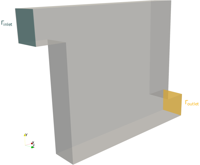
OpenFOAM simulation¶

OpenFOAM solves the steady incompressible Navier-Stokes equations in $\Omega$ :

(\mathbf{w} \cdot \nabla)\mathbf{w} - \nu \Delta \mathbf{w} + \nabla p = \mathbf{0}, \qquad \nabla \cdot \mathbf{w} = 0

(1)

with kinematic viscosity $\nu = 1.0$ m $^2$ s $^{-1}$ . The boundary conditions are:

Boundary	Condition
Inlet	Fixed velocity $\mathbf{w} = (0.1,\, 0,\, 0)$ m s $^{-1}$
Outlet	Zero-gradient pressure (natural outflow)
Walls	No-slip: $\mathbf{w} = \mathbf{0}$

The Reynolds number based on the domain height is $Re = UH/\nu = 0.1 \times 1.0 / 1.0 = 0.1$ , placing the flow firmly in the creeping-flow regime where inertia is negligible. The velocity field at the converged steady state ( $t = 11.1$ s) is used directly as $\mathbf{w}$ in the advection-diffusion problem.

Advection-diffusion equation¶

The concentration $u$ [m $^{-3}$ ] satisfies the steady advection-diffusion equation

\nabla \cdot (\mathbf{w} u - D \nabla u) = f \quad \text{in } \Omega

(2)

where $\mathbf{w}$ [m s $^{-1}$ ] is the OpenFOAM velocity field, $D = 10^{-3}$ m $^2$ s $^{-1}$ is the diffusivity, and $f = 1$ m $^{-3}$ s $^{-1}$ is a uniform volumetric source. The weak formulation and DG discretisation are identical to Examples 1--3.

Boundary conditions¶

The advection-diffusion boundary conditions follow the same pattern as Examples 1--3.

Boundary	$\mathbf{w} \cdot \mathbf{n}$	Advection	Diffusion
Inlet	$< 0$ (inflow)	Prescribed inflow: $u = 0$	Nitsche: $u = 0$
Outlet	$> 0$ (outflow)	Do-nothing: $\mathbf{w} \cdot \mathbf{n}\, u$ applied without upwind filter	Natural (zero normal flux)
Walls	$= 0$	No term	Natural (zero normal flux)

The outlet uses a do-nothing condition rather than the upwind-filtered form used in Examples 1--3. This is more robust for the 3D geometry, where the flow may have small recirculation near the outlet step.

import zipfile
from pathlib import Path

from mpi4py import MPI
from petsc4py import PETSc

import numpy as np

import ufl
import basix.ufl
import dolfinx
from dolfinx import fem
from dolfinx.fem.petsc import NonlinearProblem
import io4dolfinx
from foam2dolfinx import OpenFOAMReader

COMM = MPI.COMM_WORLD

Extracting the foam data¶

The OpenFOAM case is stored in foam_data.zip. We extract it once; if foam_data/ already exists the cell is a no-op.

if not Path("foam_data").exists():
    with zipfile.ZipFile("foam_data.zip", "r") as z:
        z.extractall(".")
    print("Extracted foam_data.zip")
else:
    print("foam_data/ already exists, skipping extraction")

foam_data/ already exists, skipping extraction

Reading the OpenFOAM data¶

The foam2dolfinx library reads the OpenFOAM case directly into DOLFINx objects. Internally it uses pyvista to parse the OpenFOAM binary, then reorders the tetrahedral connectivity to match DOLFINx’s vertex ordering and maps the node-centred velocity data from OpenFOAM onto a CG1 vector function space. The create_facet_meshtags call matches each OpenFOAM boundary patch to the corresponding DOLFINx facets and assigns integer IDs in the order the patches appear in the boundary file.

foam_file = Path("foam_data/box.foam")
time_value = 11.1

reader = OpenFOAMReader(filename=foam_file, cell_type=10)
w_foam = reader.create_dolfinx_function_with_point_data(t=time_value, name="U")
msh = reader.dolfinx_meshes_dict["default"]
facet_mt = reader.create_facet_meshtags()

INLET_ID = 1
OUTLET_ID = 2
WALLS_ID = 3

Boundary patch summary:
  inlet: id=1, n_facets=302
  outlet: id=2, n_facets=292
  walls: id=3, n_facets=22398

import pyvista

grid = pyvista.UnstructuredGrid(*dolfinx.plot.vtk_mesh(msh, msh.topology.dim))
vel = w_foam.x.array.reshape(-1, 3)
grid.point_data["U_mag"] = np.linalg.norm(vel, axis=1)
grid.point_data["U"] = vel
grid.set_active_scalars("U_mag")

surface = grid.extract_surface(algorithm="dataset_surface")

slc = grid.slice(normal=[0, 0, 1], origin=[0.7, 0.5, 0.1])
glyphs = slc.glyph(orient="U", scale="U_mag", factor=0.5)

pl = pyvista.Plotter(off_screen=True, window_size=(1000, 600))
pl.add_mesh(surface, scalars="U_mag", cmap="viridis", opacity=0.2, show_scalar_bar=False)
pl.add_mesh(slc, scalars="U_mag", cmap="viridis", scalar_bar_args={
    "title": "||w|| (m/s)",
    "vertical": False,
    "position_x": 0.25,
    "position_y": 0.02,
    "width": 0.5,
    "height": 0.05,
})
pl.add_mesh(glyphs, color="white", opacity=0.9)

pl.camera_position = [(3, 1.5, 1.0), (0.7, 0.5, 0.1), (0, 1, 0)]
pl.camera.zoom(1.2)
pl.save_graphic("velocity.svg")
pl.close()

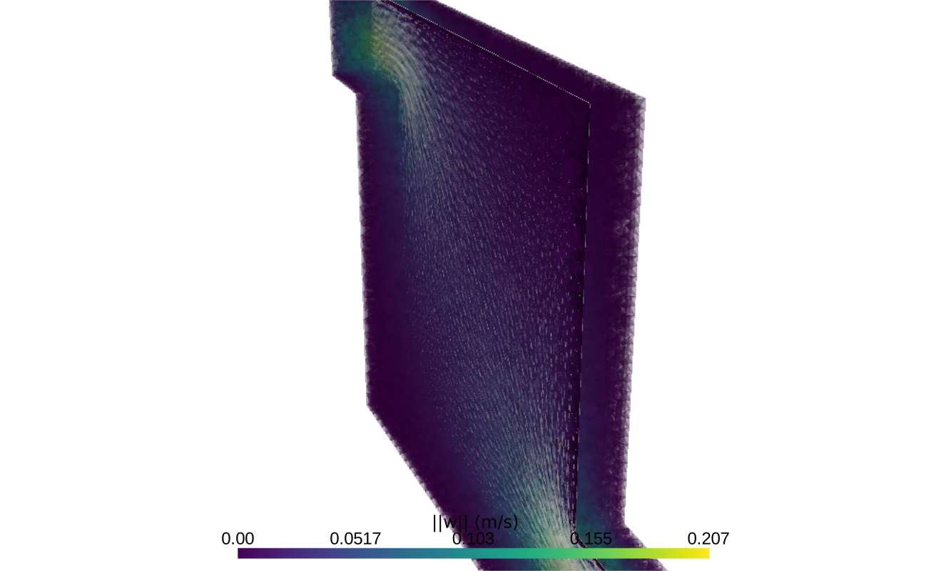
The velocity field coloured by magnitude, with the full 3D mesh visible. The flow is directed from the inlet (upper left) to the outlet (lower right).

Saving to checkpoint¶

We write the mesh, facet tags, and velocity field to an io4dolfinx checkpoint so the advection-diffusion solve can be re-run without re-reading the OpenFOAM data.

CHECKPOINT = Path("foam_data/sim_checkpoint.bp")

io4dolfinx.write_mesh(CHECKPOINT, msh)
io4dolfinx.write_function(CHECKPOINT, w_foam, time=0.0, name="U")
io4dolfinx.write_meshtags(CHECKPOINT, msh, facet_mt, meshtag_name="facet_tags")

Loading the velocity field¶

We reload the mesh, facet tags, and velocity from the checkpoint. The velocity was stored at degree 1 (CG1), matching the OpenFOAM node-centred format.

msh = io4dolfinx.read_mesh(CHECKPOINT, COMM)
msh.topology.create_connectivity(msh.topology.dim, msh.topology.dim - 1)
msh.topology.create_connectivity(msh.topology.dim - 1, msh.topology.dim)
facet_mt = io4dolfinx.read_meshtags(CHECKPOINT, msh, meshtag_name="facet_tags")

gdim = msh.geometry.dim
el = basix.ufl.element("Lagrange", msh.topology.cell_name(), 1, shape=(gdim,))
w = fem.Function(fem.functionspace(msh, el), name="U")
io4dolfinx.read_function(CHECKPOINT, w, time=0.0, name="U")

Setting up the advection-diffusion problem¶

The formulation follows Example 3. The concentration $u$ is represented as a fem.Function (rather than a TrialFunction) so that the same nonlinear solver path used in Examples 1--3 is retained. The outlet uses a do-nothing condition, applying $\mathbf{w} \cdot \mathbf{n}\, u$ without upwind filtering, which is more robust when the flow has slight recirculation near the outlet step.

V = fem.functionspace(msh, ("DG", 1))
u = fem.Function(V)
v_u = ufl.TestFunction(V)

n = ufl.FacetNormal(msh)
h = ufl.CellDiameter(msh)
ds = ufl.Measure("ds", domain=msh, subdomain_data=facet_mt)
dS, dx = ufl.dS, ufl.dx

D = fem.Constant(msh, PETSc.ScalarType(1e-3))
penalty = fem.Constant(msh, PETSc.ScalarType(200))
u_inlet = fem.Constant(msh, PETSc.ScalarType(0.0))
f_source = fem.Constant(msh, PETSc.ScalarType(1.0))
lmbda = ufl.conditional(ufl.gt(ufl.dot(w, n), 0), 1, 0)

F_outlet = ufl.inner(ufl.dot(w, n) * u, v_u) * ds(OUTLET_ID)

F_inlet = (
    D * (
        -ufl.inner(ufl.grad(u), v_u * n)
        - ufl.inner(ufl.grad(v_u), u * n)
        + (penalty / h) * ufl.inner(u, v_u)
    )
    - ufl.inner((1 - lmbda) * ufl.dot(w, n) * u_inlet, v_u)
    + D * (
        ufl.inner(ufl.grad(v_u), u_inlet * n)
        - (penalty / h) * ufl.inner(u_inlet, v_u)
    )
) * ds(INLET_ID)

F = (
    -ufl.inner(w * u, ufl.grad(v_u)) * dx
    + ufl.inner(2 * ufl.avg(lmbda * w * u), ufl.jump(v_u, n)) * dS
    + F_outlet
    + D * ufl.inner(ufl.grad(u), ufl.grad(v_u)) * dx
    - D * ufl.inner(ufl.avg(ufl.grad(u)), ufl.jump(v_u, n)) * dS
    - D * ufl.inner(ufl.jump(u, n), ufl.avg(ufl.grad(v_u))) * dS
    + D * (penalty / ufl.avg(h)) * ufl.inner(ufl.jump(u, n), ufl.jump(v_u, n)) * dS
    + F_inlet
    - ufl.inner(f_source, v_u) * dx
)

Solving¶

The nonlinear problem is passed to PETSc SNES (Scalable Nonlinear Equations Solver), which applies a Newton iteration. Because $F$ is linear in $u$ , SNES converges in a single step. The linear system is solved with MUMPS, a sparse direct solver well-suited to the unstructured 3D mesh.

problem = NonlinearProblem(
    F,
    u,
    J=ufl.derivative(F, u),
    petsc_options_prefix="adv_diff",
    petsc_options={
        "snes_atol": 1e-12,
        "snes_rtol": 1e-12,
        "snes_max_it": 30,
        "ksp_type": "preonly",
        "pc_type": "lu",
        "pc_factor_mat_solver_type": "mumps",
    },
)
u = problem.solve()
u.x.scatter_forward()

topology, cell_types, geometry = dolfinx.plot.vtk_mesh(V)
grid_u = pyvista.UnstructuredGrid(topology, cell_types, geometry)
grid_u.point_data["u"] = u.x.array
grid_u.set_active_scalars("u")

surface_u = grid_u.extract_surface(algorithm="dataset_surface")
slc_u = grid_u.slice(normal=[0, 0, 1], origin=[0.7, 0.5, 0.1])

pl = pyvista.Plotter(off_screen=True, window_size=(1000, 600))
pl.add_mesh(surface_u, scalars="u", cmap="plasma", opacity=0.2, show_scalar_bar=False)
pl.add_mesh(slc_u, scalars="u", cmap="plasma", scalar_bar_args={
    "title": "u (m^-3)",
    "vertical": False,
    "position_x": 0.25,
    "position_y": 0.02,
    "width": 0.5,
    "height": 0.05,
})
pl.view_vector([1, 1, 1], viewup=[0.2, -0.5, 0])
pl.camera.zoom(1.2)
pl.save_graphic("concentration.svg")
pl.close()

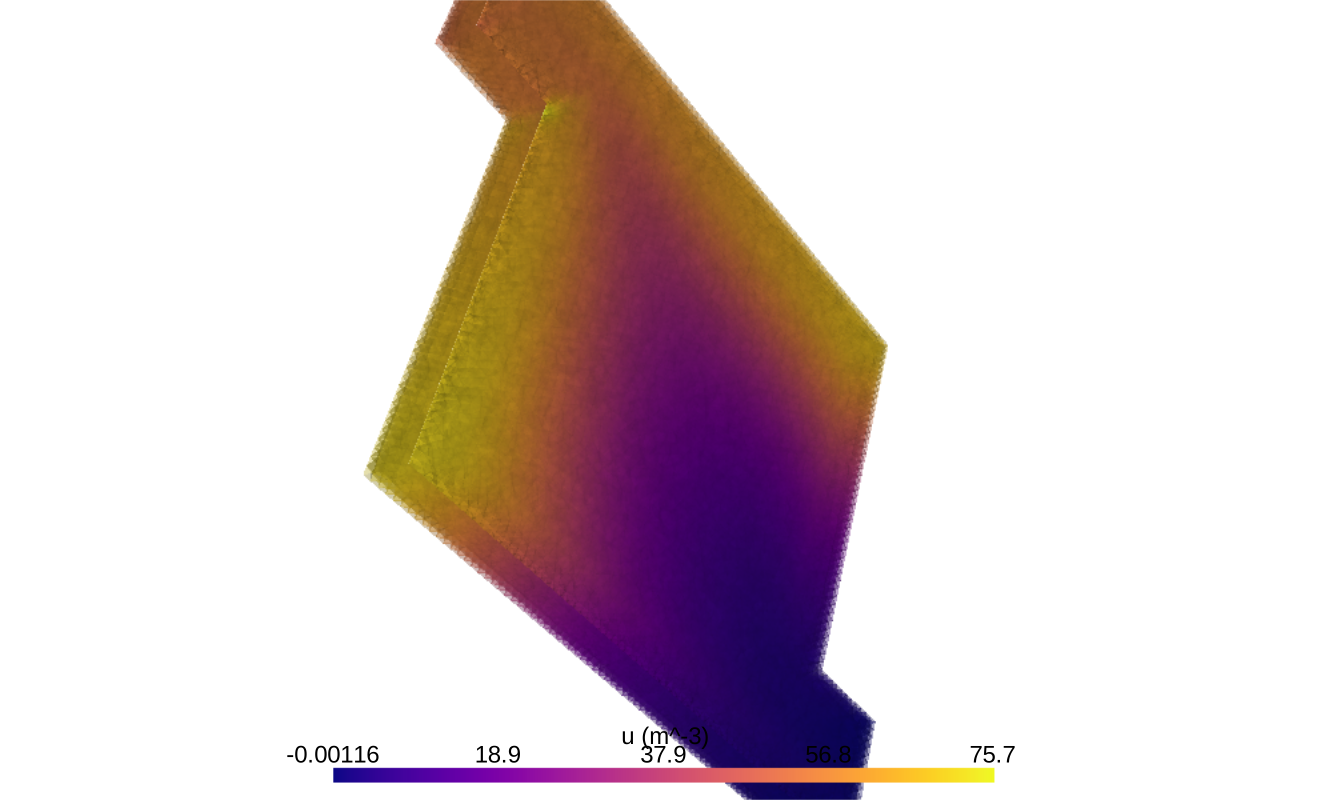
The concentration field across the full 3D mesh. The source $f = 1$ m $^{-3}$ s $^{-1}$ is active throughout the domain; concentration accumulates and is carried toward the outlet by the flow.

Flux balance verification¶

We verify the solution by computing the net flux of $u$ through each boundary using the consistent-flux approach from Examples 1--3. At steady state, the total flux leaving the domain must equal the volumetric source integral. We expect nearly all of the tracer to exit through the outlet, with negligible flux at the inlet (since $u_\text{inlet} = 0$ ) and zero flux at the walls.

R = F
R_outlet = F_outlet
R_inlet = F_inlet

tdim = msh.topology.dim
fdim = tdim - 1
msh.topology.create_connectivity(fdim, tdim)
msh.topology.create_connectivity(tdim, tdim)
owned_size = V.dofmap.index_map.size_local * V.dofmap.index_map_bs


def get_owned_dofs(marker):
    facets = facet_mt.find(marker)
    if len(facets) == 0:
        return np.array([], dtype=np.int32)
    f_to_c = msh.topology.connectivity(fdim, tdim)
    cells = np.unique(np.concatenate([f_to_c.links(f) for f in facets]))
    dofs = fem.locate_dofs_topological(V, tdim, cells)
    return dofs[dofs < owned_size]


def compute_consistent_flux(residual_form, dofs):
    residual = fem.assemble_vector(fem.form(residual_form))
    residual.scatter_reverse(dolfinx.la.InsertMode.add)
    residual.scatter_forward()
    return msh.comm.allreduce(np.sum(residual.array[dofs]), op=MPI.SUM)


flux_outlet = -compute_consistent_flux(R - R_outlet, get_owned_dofs(OUTLET_ID))
flux_inlet = -compute_consistent_flux(R - R_inlet, get_owned_dofs(INLET_ID))
flux_wall = compute_consistent_flux(R, get_owned_dofs(WALLS_ID))

source_total = COMM.allreduce(
    fem.assemble_scalar(fem.form(f_source * dx)), op=MPI.SUM
)
consist_total = flux_outlet + flux_wall + flux_inlet


def pct(val):
    return 100 * val / source_total


print(f"Source integral : {source_total:.6e}")
print()
print(f"{'Flux outlet':20s} {flux_outlet:14.6e}")
print(f"{'Flux inlet':20s} {flux_inlet:14.6e}")
print(f"{'Flux wall':20s} {flux_wall:14.6e}")
print()
c_bal = source_total - consist_total
print(f"{'Total flux':20s} {consist_total:14.6e}")
print(f"{'Balance residual':20s} {c_bal:14.6e} ({pct(c_bal):+.2f}%)")

Source integral : 2.160000e-01

Flux outlet            2.155064e-01
Flux inlet             4.935857e-04
Flux wall             -9.788433e-15

Total flux             2.160000e-01
Balance residual       9.092727e-14 (+0.00%)