Example 3: Stokes flow in a box - Advection diffusion

Example 3: Stokes flow in a box

Problem setup¶

This example builds on Examples 1 and 2 by replacing the prescribed velocity field with one computed numerically. We solve a two-stage problem on the same mesh.

Stokes flow. Solve the steady Stokes equations on the domain to obtain a divergence-free velocity field $\mathbf{w}$ .
Advection-diffusion. Solve the advection-diffusion equation using $\mathbf{w}$ as the transport velocity, with a uniform volumetric source $f = 1$ .

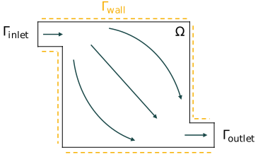
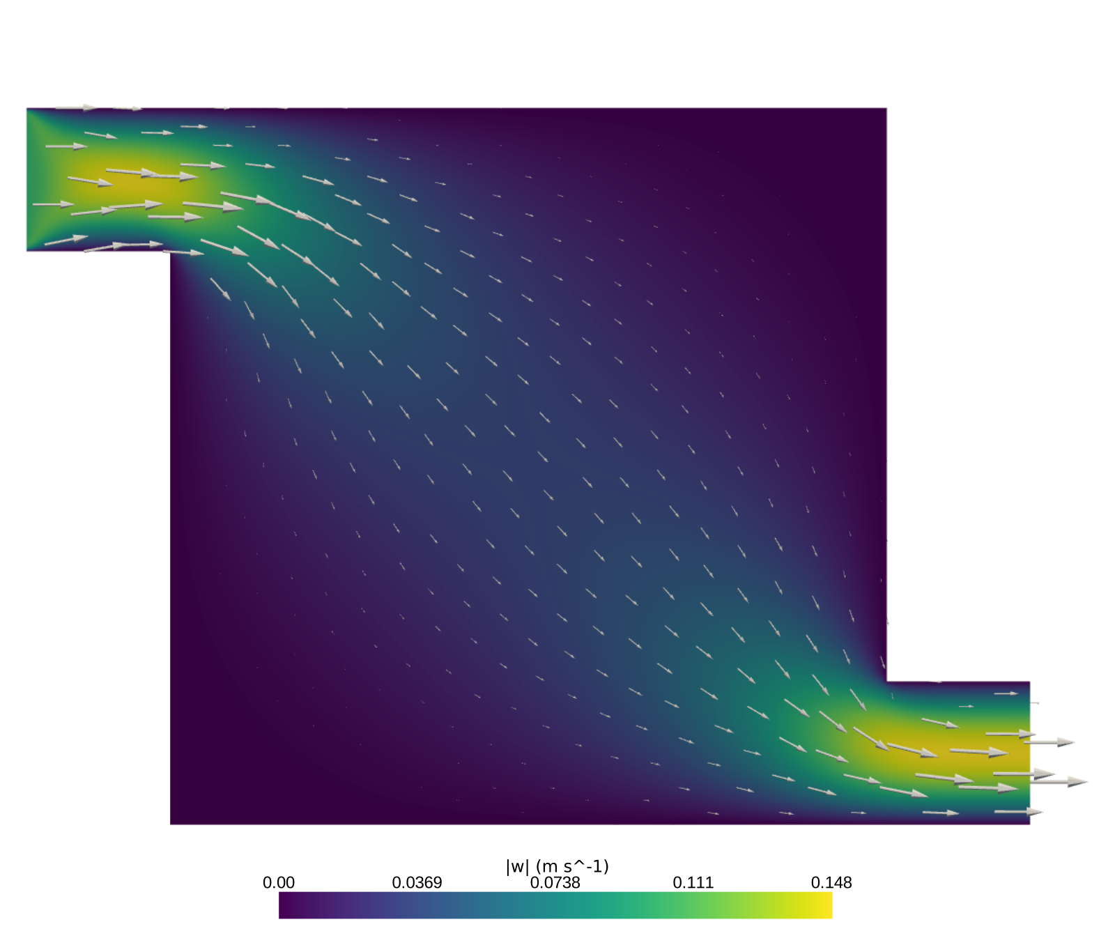
The domain $\Omega$ is a 1 × 1 box with a 0.2 × 0.2 inlet channel protruding from the top-left and a 0.2 × 0.2 outlet channel protruding from the bottom-right (both extending in the $x$ -direction). Fluid enters through the inlet and exits through the outlet, so the flow path crosses the box diagonally.

The Stokes equations¶

The Stokes equations describe viscous flow at very low Reynolds number, where inertia is negligible compared to viscosity. The strong form is

-\mu \Delta \mathbf{w} + \nabla p = \mathbf{0}, \qquad \nabla \cdot \mathbf{w} = 0 \quad \text{in } \Omega,

(1)

where $\mathbf{w}$ is the velocity, $p$ is the pressure, and $\mu$ is the dynamic viscosity (Pa s).

Discretisation. We use Taylor-Hood elements: a continuous piecewise-quadratic space (P2) for velocity and a continuous piecewise-linear space (P1) for pressure.

The weak form is: find $(\mathbf{w}, p) \in V_h \times Q_h$ such that for all $(\mathbf{v}_w, q)$ ,

\mu\int_\Omega \nabla\mathbf{w} : \nabla\mathbf{v}_w\,\mathrm{d}x - \int_\Omega p\,\nabla\cdot\mathbf{v}_w\,\mathrm{d}x - \int_\Omega (\nabla\cdot\mathbf{w})\,q\,\mathrm{d}x = 0.

(2)

The advection-diffusion equation¶

The advection-diffusion equation for the scalar concentration $u$ is

\mathbf{w} \cdot \nabla u - D \Delta u = f \quad \text{in } \Omega,

(3)

where $D$ is the diffusivity (m $^2$ s $^{-1}$ ) and $f$ is a volumetric source. The velocity field $\mathbf{w}$ is taken from the Stokes solve above rather than prescribed analytically as in Examples 1 and 2. The DG weak form, upwind advection flux, SIPG diffusion, and Nitsche inlet condition are identical to those examples.

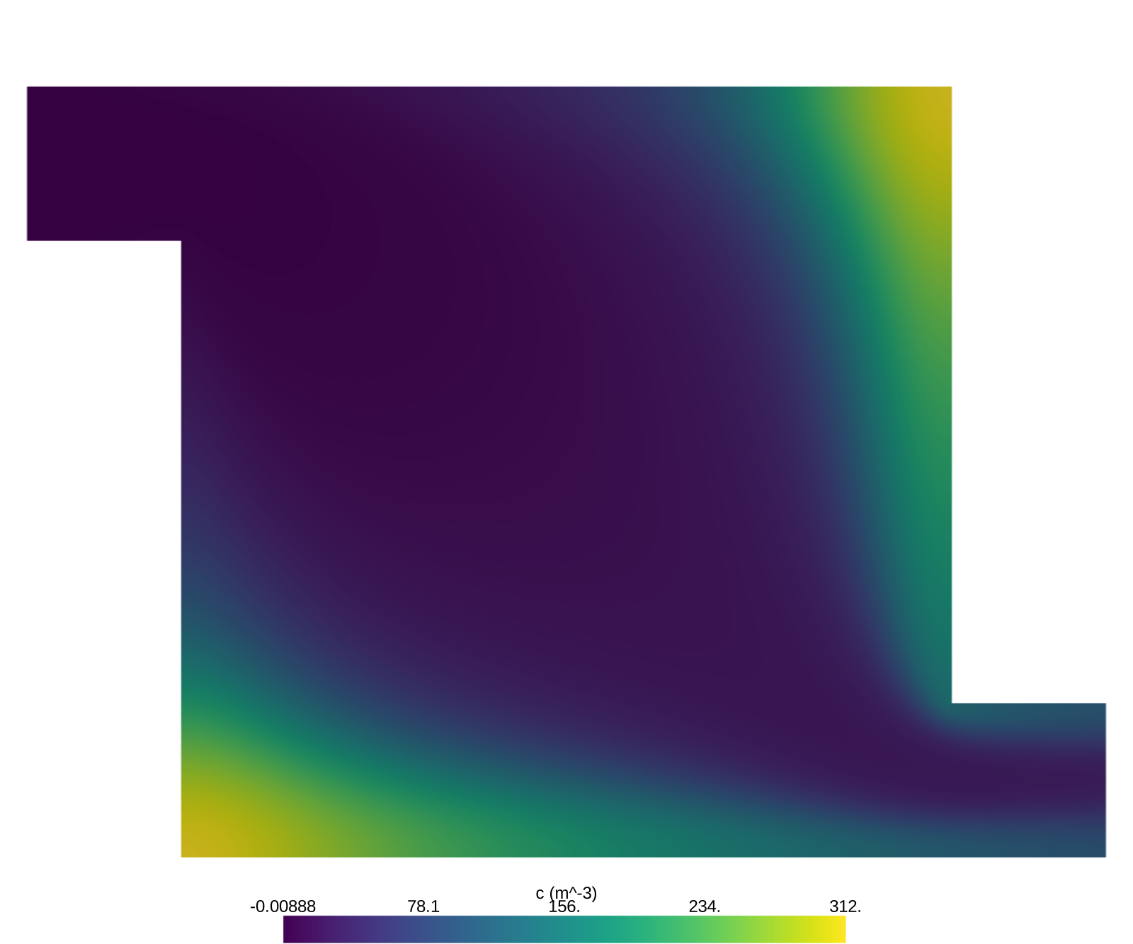
We take $D = 10^{-5}$ m $^2$ s $^{-1}$ and $f = 1$ , giving a large Péclet number so the solution is strongly advection-dominated.

Boundary conditions¶

Stokes¶

Boundary	Condition
Inlet	Plug flow: $\mathbf{w} = (0.1,\, 0)$ m s $^{-1}$ (Dirichlet)
Outlet	Natural, zero normal stress
Walls	No-slip: $\mathbf{w} = \mathbf{0}$ (Dirichlet)

The outlet condition is natural: no term is added to the weak form for that boundary, so the variational principle automatically enforces zero normal stress there.

Advection-diffusion¶

Boundary	$\mathbf{w}\cdot\mathbf{n}$	Advection	Diffusion
Inlet	$< 0$ (inflow)	Prescribed inflow: $u = 0$	Nitsche: $u = 0$
Outlet	$> 0$ (outflow)	Natural upwind outflow	Natural (zero normal flux)
Walls	$= 0$	No term	Natural (zero normal flux)

from pathlib import Path

from mpi4py import MPI
from petsc4py import PETSc

import numpy as np
import ufl
import dolfinx
from dolfinx import fem, plot
from dolfinx.fem.petsc import LinearProblem, NonlinearProblem
from dolfinx.io import XDMFFile
import io4dolfinx

COMM = MPI.COMM_WORLD

Loading the mesh¶

The mesh was generated in SALOME and saved as a .med file. We convert it to the XDMF format expected by DOLFINx using meshio. The function also returns a correspondence dictionary mapping integer boundary tags to the names assigned in SALOME, which is where the boundary IDs below come from.

import meshio


def convert_med_to_xdmf(med_file, cell_file, facet_file, cell_type, facet_type):
    msh = meshio.read(med_file)
    corr_dict = {-k: v for k, v in msh.cell_tags.items()}
    for mesh_block in msh.cells:
        if mesh_block.type == cell_type:
            meshio.write_points_cells(
                cell_file,
                msh.points,
                [mesh_block],
                cell_data={"f": [-1 * msh.cell_data_dict["cell_tags"][cell_type]]},
            )
        elif mesh_block.type == facet_type:
            meshio.write_points_cells(
                facet_file,
                msh.points,
                [mesh_block],
                cell_data={"f": [-1 * msh.cell_data_dict["cell_tags"][facet_type]]},
            )
    return corr_dict


corr_dict = convert_med_to_xdmf(
    med_file="mesh_data/box_mesh.med",
    cell_file="mesh_data/mesh_domains.xdmf",
    facet_file="mesh_data/mesh_boundaries.xdmf",
    cell_type="triangle",
    facet_type="line",
)
print(corr_dict)

INLET_ID = 7
OUTLET_ID = 8
WALLS_ID = 9

with XDMFFile(COMM, "mesh_data/mesh_domains.xdmf", "r") as f:
    msh = f.read_mesh(name="Grid")
msh.topology.create_connectivity(msh.topology.dim, msh.topology.dim - 1)
msh.topology.create_connectivity(msh.topology.dim - 1, msh.topology.dim)
with XDMFFile(COMM, "mesh_data/mesh_boundaries.xdmf", "r") as f:
    facet_mt = f.read_meshtags(msh, name="Grid")

{np.int64(6): ['fluid'], np.int64(7): ['inlet'], np.int64(8): ['outlet'], np.int64(9): ['walls']}

Solving Stokes flow¶

We set up the Taylor-Hood function space and apply boundary conditions as described above. After solving, the velocity sub-solution is extracted into a standalone CG2 vector field.

import basix.ufl

gdim = msh.geometry.dim
fdim = msh.topology.dim - 1

P2 = basix.ufl.element("Lagrange", msh.topology.cell_name(), 2, shape=(gdim,))
P1 = basix.ufl.element("Lagrange", msh.topology.cell_name(), 1)
W = fem.functionspace(msh, basix.ufl.mixed_element([P2, P1]))
V_sub, _ = W.sub(0).collapse()

w_in = fem.Function(V_sub)
w_in.interpolate(
    lambda x: np.vstack([0.1 * np.ones(x.shape[1]), np.zeros(x.shape[1])])
)
bcs = [
    fem.dirichletbc(
        w_in,
        fem.locate_dofs_topological(
            (W.sub(0), V_sub), fdim, facet_mt.find(INLET_ID)
        ),
        W.sub(0),
    ),
    fem.dirichletbc(
        fem.Function(V_sub),
        fem.locate_dofs_topological(
            (W.sub(0), V_sub), fdim, facet_mt.find(WALLS_ID)
        ),
        W.sub(0),
    ),
]

w_tr, p_tr = ufl.TrialFunctions(W)
v_w, q = ufl.TestFunctions(W)
mu = fem.Constant(msh, PETSc.ScalarType(1.0))
a = (
    mu * ufl.inner(ufl.grad(w_tr), ufl.grad(v_w)) * ufl.dx
    - ufl.inner(p_tr, ufl.div(v_w)) * ufl.dx
    - ufl.inner(ufl.div(w_tr), q) * ufl.dx
)
L = ufl.inner(fem.Constant(msh, PETSc.ScalarType((0.0,) * gdim)), v_w) * ufl.dx

stokes_problem = LinearProblem(
    a,
    L,
    bcs=bcs,
    petsc_options_prefix="stokes",
    petsc_options={
        "ksp_type": "preonly",
        "pc_type": "lu",
        "pc_factor_mat_solver_type": "mumps",
        "ksp_error_if_not_converged": True,
    },
)
wh = stokes_problem.solve()

el_cg2 = basix.ufl.element("Lagrange", msh.topology.cell_name(), 2, shape=(gdim,))
V_cg2 = fem.functionspace(msh, el_cg2)
w_h = fem.Function(V_cg2, name="velocity")
w_h.interpolate(wh.sub(0).collapse())
w_h.x.scatter_forward()

import pyvista

topology, cell_types, geometry = plot.vtk_mesh(V_cg2)
w_grid = pyvista.UnstructuredGrid(topology, cell_types, geometry)
w_values = w_h.x.array.reshape(-1, gdim)
w_3d = np.zeros((w_values.shape[0], 3))
w_3d[:, :gdim] = w_values
w_grid["w"] = w_3d
w_grid["w_mag"] = np.linalg.norm(w_values, axis=1)

glyphs = w_grid.glyph(orient="w", scale="w_mag", factor=0.6, tolerance=0.03)

plotter = pyvista.Plotter(off_screen=True, window_size=(1200, 1000))
field_actor = plotter.add_mesh(
    w_grid, scalars="w_mag", cmap="viridis", show_scalar_bar=False
)
plotter.add_mesh(glyphs, color="white", show_scalar_bar=False)
plotter.add_scalar_bar(
    title="|w| (m s^-1)",
    mapper=field_actor.mapper,
    vertical=False,
    width=0.5,
    height=0.08,
    position_x=0.25,
    position_y=0.01,
)
plotter.view_xy()
plotter.camera.tight(padding=0.05, adjust_render_window=False)
plotter.save_graphic("velocity_field_mwe3.svg")
plotter.close()

Saving to checkpoint¶

We use io4dolfinx to write the mesh, facet tags, and velocity to a checkpoint file. This separates the Stokes solve from the advection-diffusion solve, so the transport problem can be re-run with different parameters, for example a different diffusivity, without repeating the Stokes computation.

CHECKPOINT = Path("sim_checkpoint.bp")

io4dolfinx.write_mesh(CHECKPOINT, msh)
io4dolfinx.write_meshtags(CHECKPOINT, msh, facet_mt, meshtag_name="facets")
io4dolfinx.write_function(CHECKPOINT, w_h, time=0.0, name="velocity")

Loading the velocity field¶

We reload the mesh, facet tags, and Stokes velocity from the checkpoint. From this point the advection-diffusion solve is entirely independent of the Stokes solve, requiring only the velocity field stored in the checkpoint.

msh = io4dolfinx.read_mesh(CHECKPOINT, COMM)
msh.topology.create_connectivity(msh.topology.dim, msh.topology.dim - 1)
msh.topology.create_connectivity(msh.topology.dim - 1, msh.topology.dim)
facet_mt = io4dolfinx.read_meshtags(CHECKPOINT, msh, meshtag_name="facets")

gdim = msh.geometry.dim
el_cg2 = basix.ufl.element("Lagrange", msh.topology.cell_name(), 2, shape=(gdim,))
V_cg2 = fem.functionspace(msh, el_cg2)
w = fem.Function(V_cg2, name="velocity")
io4dolfinx.read_function(CHECKPOINT, w, time=0.0, name="velocity")

Setting up the advection-diffusion problem¶

We use a DG1 function space for the concentration $u$ . The upwind indicator $\lambda$ classifies each face as outflow ( $\lambda = 1$ ) or inflow ( $\lambda = 0$ ) based on the sign of $\mathbf{w}\cdot\mathbf{n}$ , following the same pattern as Examples 1 and 2.

V = fem.functionspace(msh, ("DG", 1))
u = fem.Function(V)
v_u = ufl.TestFunction(V)

n = ufl.FacetNormal(msh)
h = ufl.CellDiameter(msh)
ds = ufl.Measure("ds", domain=msh, subdomain_data=facet_mt)
dS, dx = ufl.dS, ufl.dx

D = fem.Constant(msh, PETSc.ScalarType(1e-4))
penalty = fem.Constant(msh, PETSc.ScalarType(10))
u_inlet = fem.Constant(msh, PETSc.ScalarType(0.0))
f_source = fem.Constant(msh, PETSc.ScalarType(1.0))

lmbda = ufl.conditional(ufl.gt(ufl.dot(w, n), 0), 1, 0)

Assembling the weak form¶

The residual $F$ is assembled in the same parts as in Examples 1 and 2: advection bulk and interface terms, SIPG diffusion, the Nitsche inlet condition, and the volumetric source. The named variables F_inlet_adv, F_outlet_surf, and F_inlet_nitsche are kept so that the flux verification step can isolate individual boundary contributions.

# Advection: bulk and interior upwind flux
F = -ufl.inner(w * u, ufl.grad(v_u)) * dx
F += ufl.inner(2 * ufl.avg(lmbda * w * u), ufl.jump(v_u, n)) * dS

# Advection: boundary terms (kept named for flux verification)
F_inlet_adv = -ufl.inner((1 - lmbda) * ufl.dot(w, n) * u_inlet, v_u) * ds(INLET_ID)
F_outlet_surf = ufl.inner(lmbda * ufl.dot(w, n) * u, v_u) * ds(OUTLET_ID)
F += F_inlet_adv + F_outlet_surf

# Diffusion (SIPG): bulk and interior interface terms
F += D * ufl.inner(ufl.grad(u), ufl.grad(v_u)) * dx
F += -D * ufl.inner(ufl.avg(ufl.grad(u)), ufl.jump(v_u, n)) * dS
F += -D * ufl.inner(ufl.jump(u, n), ufl.avg(ufl.grad(v_u))) * dS
F += D * (penalty / ufl.avg(h)) * ufl.inner(ufl.jump(u, n), ufl.jump(v_u, n)) * dS

# Nitsche inlet condition (weak Dirichlet)
F_inlet_nitsche = D * (
    -ufl.inner(ufl.grad(u), v_u * n) * ds(INLET_ID)
    - ufl.inner(ufl.grad(v_u), (u - u_inlet) * n) * ds(INLET_ID)
    + (penalty / h) * ufl.inner(u - u_inlet, v_u) * ds(INLET_ID)
)
F += F_inlet_nitsche
F_inlet_terms = F_inlet_adv + F_inlet_nitsche

# Volumetric source
F += -ufl.inner(f_source, v_u) * dx

Solving¶

We solve the advection-diffusion problem and export the concentration field as a PNG.

adv_diff_problem = NonlinearProblem(
    F,
    u,
    J=ufl.derivative(F, u),
    petsc_options_prefix="adv_diff",
    petsc_options={
        "snes_atol": 1e-12,
        "snes_rtol": 1e-12,
        "snes_max_it": 30,
        "ksp_type": "preonly",
        "pc_type": "lu",
        "pc_factor_mat_solver_type": "mumps",
    },
)
u = adv_diff_problem.solve()
u.x.scatter_forward()

topology, cell_types, geometry = plot.vtk_mesh(u.function_space)
u_grid = pyvista.UnstructuredGrid(topology, cell_types, geometry)
u_grid["u"] = u.x.array

plotter = pyvista.Plotter(off_screen=True, window_size=(1200, 1000))
field_actor = plotter.add_mesh(u_grid, scalars="u", cmap="viridis", show_scalar_bar=False)
plotter.add_scalar_bar(
    title="c (m^-3)",
    mapper=field_actor.mapper,
    vertical=False,
    width=0.5,
    height=0.08,
    position_x=0.25,
    position_y=0.0,
)
plotter.view_xy()
plotter.camera.tight(padding=0.05, adjust_render_window=False)
plotter.save_graphic("concentration_mwe3.svg")
plotter.close()

Flux balance verification¶

We use the consistent-flux technique to verify global mass conservation. For each boundary, we assemble the full residual vector and sum the entries belonging to cells adjacent to that boundary. If the method is conservative, the total boundary flux should equal the volumetric source integral to machine precision.

Expected results:

Outlet flux $\approx$ source integral, most tracer leaves through the outlet.
Inlet flux $\approx 0$ , the inlet concentration is zero so no tracer enters by diffusion.
Wall flux $\approx 0$ , the natural BC gives zero normal diffusive flux and $\mathbf{w}\cdot\mathbf{n} = 0$ at no-slip walls removes advective transport.

tdim = msh.topology.dim
fdim = tdim - 1
msh.topology.create_connectivity(fdim, tdim)
msh.topology.create_connectivity(tdim, tdim)
owned_size = V.dofmap.index_map.size_local * V.dofmap.index_map_bs


def get_owned_dofs(marker):
    facets = facet_mt.find(marker)
    f_to_c = msh.topology.connectivity(fdim, tdim)
    cells = np.unique(np.concatenate([f_to_c.links(f) for f in facets]))
    dofs = fem.locate_dofs_topological(V, tdim, cells)
    return dofs[dofs < owned_size]


def compute_consistent_flux(residual_form, dofs):
    residual = fem.assemble_vector(residual_form)
    residual.scatter_reverse(dolfinx.la.InsertMode.add)
    residual.scatter_forward()
    local_flux = np.sum(residual.array[dofs])
    return msh.comm.allreduce(local_flux, op=MPI.SUM)


inlet_dofs = get_owned_dofs(INLET_ID)
outlet_dofs = get_owned_dofs(OUTLET_ID)
wall_dofs = get_owned_dofs(WALLS_ID)

F_no_outlet = fem.form(F - F_outlet_surf)
F_no_inlet = fem.form(F - F_inlet_terms)
F_form = fem.form(F)

flux_outlet = -compute_consistent_flux(F_no_outlet, outlet_dofs)
flux_inlet = -compute_consistent_flux(F_no_inlet, inlet_dofs)
flux_wall = compute_consistent_flux(F_form, wall_dofs)

source_total = msh.comm.allreduce(
    fem.assemble_scalar(fem.form(f_source * dx)), op=MPI.SUM
)

consist_total = flux_outlet + flux_wall + flux_inlet


def pct(val):
    return 100 * val / source_total


print(f"Source integral : {source_total:.6e}")
print()
print(f"{'Flux outlet':20s} {flux_outlet:14.6e}")
print(f"{'Flux inlet':20s} {flux_inlet:14.6e}")
print(f"{'Flux wall':20s} {flux_wall:14.6e}")
print()
c_bal = source_total - consist_total
print(f"{'Total flux':20s} {consist_total:14.6e}")
print(f"{'Balance residual':20s} {c_bal:14.6e} ({pct(c_bal):+.2f}%)")

Source integral : 1.080000e+00

Flux outlet            1.079791e+00
Flux inlet             2.085499e-04
Flux wall              4.880354e-16

Total flux             1.080000e+00
Balance residual       5.107026e-15 (+0.00%)